一文搞懂Python Sklearn库使用

目录1、LabelEncoder2、OneHotEncoder3、sklearn.model_selection.train_test_split随机划分训练集和测试集4、pipeline5 perdict 直接返回预测值6 sklearn.metrics中的评估方法7 GridSearchCV8 StandardScaler9 PolynomialFeatures4、10+款机器学习算法对比4.1 生成数据4.2 八款主流机器学习模型4.3 树模型 - 随机森林4.4 一些结果展示：每个模型的准确率与召回率4.5 结果展示：校准曲线4.6 模型的结果展示：重要性输出4.7 ROC值的计算与plot

Python sklearn库是一个丰富的机器学习库，里面包含内容太多，这里对一些工程里常用的操作做个简要的概述，以后还会根据自己用的进行更新。

1、LabelEncoder

简单来说 LabelEncoder 是对不连续的数字或者文本进行按序编号，可以用来生成属性/标签

from sklearn.preprocessing import LabelEncoderencoder=LabelEncoder()encoder.fit([1,3,2,6])t=encoder.transform([1,6,6,2])print(t)

输出： [0 3 3 1]

2、OneHotEncoder

OneHotEncoder 用于将表示分类的数据扩维，将[[1]，[2]，[3]，[4]]映射为 0,1,2,3的位置为1（高维的数据自己可以测试）：

from sklearn.preprocessing import OneHotEncoderoneHot=OneHotEncoder()#声明一个编码器oneHot.fit([[1],[2],[3],[4]])print(oneHot.transform([[2],[3],[1],[4]]).toarray())

输出：[[0. 1. 0. 0.]
[0. 0. 1. 0.]
[1. 0. 0. 0.]
[0. 0. 0. 1.]]
正如keras中的keras.utils.to_categorical(y_train, num_classes)

3、sklearn.model_selection.train_test_split随机划分训练集和测试集

一般形式：
train_test_split是交叉验证中常用的函数，功能是从样本中随机的按比例选取train data和testdata，形式为：

X_train,X_test, y_train, y_test =train_test_split(train_data,train_target,test_size=0.2, train_size=0.8,random_state=0)

参数解释：
- train_data：所要划分的样本特征集
- train_target：所要划分的样本结果
- test_size：测试样本占比，如果是整数的话就是样本的数量

-train_size：训练样本的占比，（注：测试占比和训练占比任写一个就行）
- random_state：是随机数的种子。
- 随机数种子：其实就是该组随机数的编号，在需要重复试验的时候，保证得到一组一样的随机数。比如你每次都填1，其他参数一样的情况下你得到的随机数组是一样的。但填0或不填，每次都会不一样。
随机数的产生取决于种子，随机数和种子之间的关系遵从以下两个规则：
- 种子不同，产生不同的随机数；种子相同，即使实例不同也产生相同的随机数。

from sklearn.model_selection import train_test_splitfrom sklearn.datasets import load_irisiris=load_iris()train=iris.datatarget=iris.target# 避免过拟合，采用交叉验证，验证集占训练集20%，固定随机种子（random_state)train_X,test_X, train_y, test_y = train_test_split(train, target, test_size = 0.2, random_state = 0)print(train_y.shape)

得到的结果数据：train_X : 训练集的数据,train_Y：训练集的标签，对应test 为测试集的数据和标签

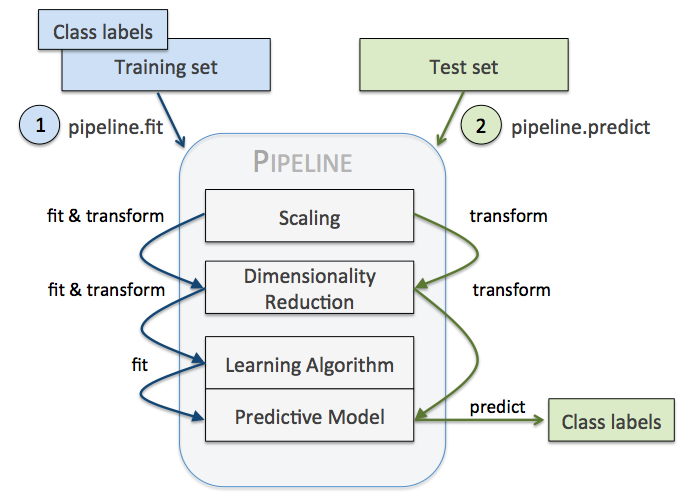
4、pipeline

本节参考与文章：用 Pipeline 将训练集参数重复应用到测试集
pipeline 实现了对全部步骤的流式化封装和管理，可以很方便地使参数集在新数据集上被重复使用。

pipeline 可以用于下面几处：

模块化 Feature Transform，只需写很少的代码就能将新的 Feature 更新到训练集中。 自动化 Grid Search，只要预先设定好使用的 Model 和参数的候选，就能自动搜索并记录最佳的 Model。 自动化 Ensemble Generation，每隔一段时间将现有最好的 K 个 Model 拿来做 Ensemble。

问题是要对数据集 Breast Cancer Wisconsin 进行分类，
该数据集包含 569 个样本，第一列 ID，第二列类别(M=恶性肿瘤，B=良性肿瘤)，
第 3-32 列是实数值的特征。

我们要用 Pipeline 对训练集和测试集进行如下操作：

先用 StandardScaler 对数据集每一列做标准化处理，（是 transformer） 再用 PCA 将原始的 30 维度特征压缩的 2 维度，（是 transformer） 最后再用模型 LogisticRegression。（是 Estimator） 调用 Pipeline 时，输入由元组构成的列表，每个元组第一个值为变量名，元组第二个元素是 sklearn 中的 transformer 或 Estimator。

注意中间每一步是 transformer，即它们必须包含 fit 和 transform 方法，或者 fit_transform。
最后一步是一个 Estimator，即最后一步模型要有 fit 方法，可以没有 transform 方法。

然后用 Pipeline.fit对训练集进行训练，pipe_lr.fit(X_train, y_train)
再直接用 Pipeline.score 对测试集进行预测并评分 pipe_lr.score(X_test, y_test)

import pandas as pdfrom sklearn.model_selection import train_test_splitfrom sklearn.preprocessing import LabelEncoderfrom sklearn.preprocessing import StandardScalerfrom sklearn.decomposition import PCAfrom sklearn.linear_model import LogisticRegression from sklearn.pipeline import Pipeline#需要联网df = pd.read_csv(’http://archive.ics.uci.edu/ml/machine-learning-databases/breast-cancer-wisconsin/wdbc.data’, header=None) # Breast Cancer Wisconsin datasetX, y = df.values[:, 2:], df.values[:, 1]encoder = LabelEncoder()y = encoder.fit_transform(y)X_train, X_test, y_train, y_test = train_test_split(X, y, test_size=.2, random_state=0)pipe_lr = Pipeline([(’sc’, StandardScaler()), (’pca’, PCA(n_components=2)), (’clf’, LogisticRegression(random_state=1)) ])pipe_lr.fit(X_train, y_train)print(’Test accuracy: %.3f’ % pipe_lr.score(X_test, y_test))

还可以用来选择特征：

例如用 SelectKBest 选择特征，
分类器为 SVM，

anova_filter = SelectKBest(f_regression, k=5)clf = svm.SVC(kernel=’linear’)anova_svm = Pipeline([(’anova’, anova_filter), (’svc’, clf)])

当然也可以应用 K-fold cross validation：

Pipeline 的工作方式：

当管道 Pipeline 执行 fit 方法时，
首先 StandardScaler 执行 fit 和 transform 方法，
然后将转换后的数据输入给 PCA，
PCA 同样执行 fit 和 transform 方法，
再将数据输入给 LogisticRegression，进行训练。

5 perdict 直接返回预测值

predict_proba返回每组数据预测值的概率，每行的概率和为1，如训练集/测试集有 下例中的两个类别，测试集有三个，则 predict返回的是一个 3*1的向量，而 predict_proba 返回的是 3*2维的向量，如下结果所示。

# conding :utf-8from sklearn.linear_model import LogisticRegressionimport numpy as np x_train = np.array([[1, 2, 3], [1, 3, 4], [2, 1, 2], [4, 5, 6], [3, 5, 3], [1, 7, 2]]) y_train = np.array([3, 3, 3, 2, 2, 2]) x_test = np.array([[2, 2, 2], [3, 2, 6], [1, 7, 4]]) clf = LogisticRegression()clf.fit(x_train, y_train) # 返回预测标签print(clf.predict(x_test)) # 返回预测属于某标签的概率print(clf.predict_proba(x_test))

6 sklearn.metrics中的评估方法

1. sklearn.metrics.roc_curve(true_y. pred_proba_score, pos_labal)

计算roc曲线，roc曲线有三个属性：fpr, tpr,和阈值，因此该函数返回这三个变量,l

2. sklearn.metrics.auc(x, y, reorder=False):

计算AUC值，其中x,y分别为数组形式，根据(xi, yi)在坐标上的点，生成的曲线，然后计算AUC值；

import numpy as npfrom sklearn.metrics import roc_curvefrom sklearn.metrics import aucy = np.array([1,0,2,2])pred = np.array([0.1, 0.4, 0.35, 0.8])fpr, tpr, thresholds = roc_curve(y, pred, pos_label=2)print(tpr)print(fpr)print(thresholds)print(auc(fpr, tpr))

3. sklearn.metrics.roc_auc_score(true_y, pred_proba_y)

直接根据真实值（必须是二值）、预测值（可以是0/1, 也可以是proba值）计算出auc值，中间过程的roc计算省略

7 GridSearchCV

GridSearchCV，它存在的意义就是自动调参，只要把参数输进去，就能给出最优化的结果和参数。但是这个方法适合于小数据集，一旦数据的量级上去了，很难得出结果。这个时候就是需要动脑筋了。数据量比较大的时候可以使用一个快速调优的方法——坐标下降。它其实是一种贪心算法：拿当前对模型影响最大的参数调优，直到最优化；再拿下一个影响最大的参数调优，如此下去，直到所有的参数调整完毕。这个方法的缺点就是可能会调到局部最优而不是全局最优，但是省时间省力，巨大的优势面前，还是试一试吧，后续可以再拿bagging再优化。

回到sklearn里面的GridSearchCV，GridSearchCV用于系统地遍历多种参数组合，通过交叉验证确定最佳效果参数。

GridSearchCV的sklearn官方网址：http://scikit-learn.org/stable/modules/generated/sklearn.model_selection.GridSearchCV.html#sklearn.model_selection.GridSearchCV

classsklearn.model_selection.GridSearchCV(estimator,param_grid, scoring=None, fit_params=None, n_jobs=1, iid=True, refit=True,cv=None, verbose=0, pre_dispatch=’2*n_jobs’, error_score=’raise’,return_train_score=True)

常用参数解读

estimator：所使用的分类器，如estimator=RandomForestClassifier(min_samples_split=100,min_samples_leaf=20,max_depth=8,max_features=’sqrt’,random_state=10), 并且传入除需要确定最佳的参数之外的其他参数。每一个分类器都需要一个scoring参数，或者score方法。

param_grid：值为字典或者列表，即需要最优化的参数的取值，param_grid =param_test1，param_test1 = {’n_estimators’:range(10,71,10)}。

scoring :准确度评价标准，默认None,这时需要使用score函数；或者如scoring=’roc_auc’，根据所选模型不同，评价准则不同。字符串（函数名），或是可调用对象，需要其函数签名形如：scorer(estimator, X, y)；如果是None，则使用estimator的误差估计函数。

cv :交叉验证参数，默认None，使用三折交叉验证。指定fold数量，默认为3，也可以是yield训练/测试数据的生成器。

refit :默认为True,程序将会以交叉验证训练集得到的最佳参数，重新对所有可用的训练集与开发集进行，作为最终用于性能评估的最佳模型参数。即在搜索参数结束后，用最佳参数结果再次fit一遍全部数据集。

iid:默认True,为True时，默认为各个样本fold概率分布一致，误差估计为所有样本之和，而非各个fold的平均。

verbose：日志冗长度，int：冗长度，0：不输出训练过程，1：偶尔输出，>1：对每个子模型都输出。

n_jobs: 并行数，int：个数,-1：跟CPU核数一致, 1:默认值。

pre_dispatch：指定总共分发的并行任务数。当n_jobs大于1时，数据将在每个运行点进行复制，这可能导致OOM，而设置pre_dispatch参数，则可以预先划分总共的job数量，使数据最多被复制pre_dispatch次

进行预测的常用方法和属性

grid.fit()：运行网格搜索

grid_scores_：给出不同参数情况下的评价结果

best_params_：描述了已取得最佳结果的参数的组合

best_score_：成员提供优化过程期间观察到的最好的评分

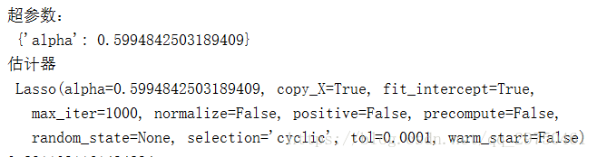
model=Lasso()alpha_can=np.logspace(-3,2,10)np.set_printoptions(suppress=True)#设置打印选项print("alpha_can=",alpha_can)#cv :交叉验证参数，默认None 这里为5折交叉# param_grid：值为字典或者列表，即需要最优化的参数的取值lasso_model=GridSearchCV(model,param_grid={’alpha’:alpha_can},cv=5)#得到最好的参数lasso_model.fit(x_train,y_train)print(’超参数：n’,lasso_model.best_params_)print("估计器n",lasso_model.best_estimator_)

如果有transform,使用Pipeline简化系统搭建流程，将transform与分类器串联起来（Pipelineof transforms with a final estimator）

pipeline= Pipeline([("features", combined_features), ("svm", svm)]) param_grid= dict(features__pca__n_components=[1, 2, 3], features__univ_select__k=[1,2], svm__C=[0.1, 1, 10]) grid_search= GridSearchCV(pipeline, param_grid=param_grid, verbose=10) grid_search.fit(X,y) print(grid_search.best_estimator_)

8 StandardScaler

作用：去均值和方差归一化。且是针对每一个特征维度来做的，而不是针对样本。

【注意：】
并不是所有的标准化都能给estimator带来好处。

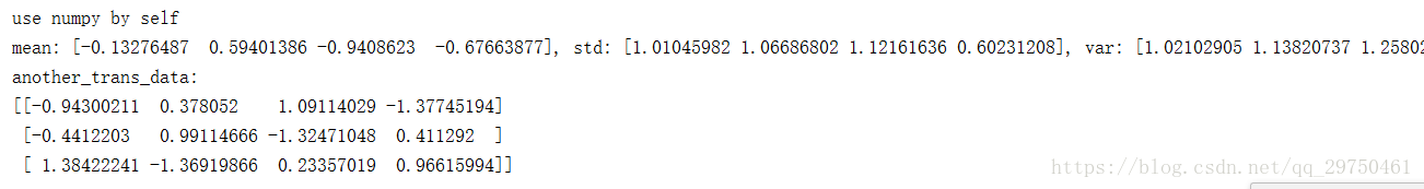
# coding=utf-8# 统计训练集的 mean 和　std 信息from sklearn.preprocessing import StandardScalerimport numpy as np def test_algorithm(): np.random.seed(123) print(’use StandardScaler’) # 注：shape of data: [n_samples, n_features] data = np.random.randn(3, 4) scaler = StandardScaler() scaler.fit(data) trans_data = scaler.transform(data) print(’original data: ’) print(data) print(’transformed data: ’) print(trans_data) print(’scaler info: scaler.mean_: {}, scaler.var_: {}’.format(scaler.mean_, scaler.var_)) print(’n’) print(’use numpy by self’) mean = np.mean(data, axis=0) std = np.std(data, axis=0) var = std * std print(’mean: {}, std: {}, var: {}’.format(mean, std, var)) # numpy 的广播功能 another_trans_data = data - mean # 注：是除以标准差 another_trans_data = another_trans_data / std print(’another_trans_data: ’) print(another_trans_data) if __name__ == ’__main__’: test_algorithm()

运行结果：

9 PolynomialFeatures

使用sklearn.preprocessing.PolynomialFeatures来进行特征的构造。

它是使用多项式的方法来进行的，如果有a，b两个特征，那么它的2次多项式为（1,a,b,a^2,ab, b^2）。

PolynomialFeatures有三个参数

degree：控制多项式的度

interaction_only： 默认为False，如果指定为True，那么就不会有特征自己和自己结合的项，上面的二次项中没有a^2和b^2。

include_bias：默认为True。如果为True的话，那么就会有上面的 1那一项。

import pandas as pdfrom sklearn.neighbors import KNeighborsClassifierfrom sklearn.model_selection import GridSearchCVfrom sklearn.pipeline import Pipeline path = r"activity_recognizer1.csv"# 数据在https://archive.ics.uci.edu/ml/datasets/Activity+Recognition+from+Single+Chest-Mounted+Accelerometerdf = pd.read_csv(path, header=None)df.columns = [’index’, ’x’, ’y’, ’z’, ’activity’] knn = KNeighborsClassifier()knn_params = {’n_neighbors’: [3, 4, 5, 6]}X = df[[’x’, ’y’, ’z’]]y = df[’activity’] from sklearn.preprocessing import PolynomialFeatures poly = PolynomialFeatures(degree=2, include_bias=False, interaction_only=False)X_ploly = poly.fit_transform(X)X_ploly_df = pd.DataFrame(X_ploly, columns=poly.get_feature_names())print(X_ploly_df.head())

运行结果：

x0 x1 x2 x0^2 x0 x1 x0 x2 x1^2
0 1502.0 2215.0 2153.0 2256004.0 3326930.0 3233806.0 4906225.0
1 1667.0 2072.0 2047.0 2778889.0 3454024.0 3412349.0 4293184.0
2 1611.0 1957.0 1906.0 2595321.0 3152727.0 3070566.0 3829849.0
3 1601.0 1939.0 1831.0 2563201.0 3104339.0 2931431.0 3759721.0
4 1643.0 1965.0 1879.0 2699449.0 3228495.0 3087197.0 3861225.0

x1 x2 x2^2
0 4768895.0 4635409.0
1 4241384.0 4190209.0
2 3730042.0 3632836.0
3 3550309.0 3352561.0
4 3692235.0 3530641.0

4、10+款机器学习算法对比

Sklearn API：http://scikit-learn.org/stable/modules/classes.html#module-sklearn.ensemble

4.1 生成数据

import numpy as npnp.random.seed(10)%matplotlib inline import matplotlib.pyplot as pltimport pandas as pdfrom sklearn.datasets import make_classificationfrom sklearn.linear_model import LogisticRegressionfrom sklearn.ensemble import (RandomTreesEmbedding, RandomForestClassifier, GradientBoostingClassifier)from sklearn.preprocessing import OneHotEncoderfrom sklearn.model_selection import train_test_splitfrom sklearn.metrics import roc_curve,accuracy_score,recall_scorefrom sklearn.pipeline import make_pipelinefrom sklearn.calibration import calibration_curveimport copyprint(__doc__)from matplotlib.colors import ListedColormapfrom sklearn.model_selection import train_test_splitfrom sklearn.preprocessing import StandardScalerfrom sklearn.datasets import make_moons, make_circles, make_classificationfrom sklearn.neural_network import MLPClassifierfrom sklearn.neighbors import KNeighborsClassifierfrom sklearn.svm import SVCfrom sklearn.gaussian_process import GaussianProcessClassifierfrom sklearn.gaussian_process.kernels import RBFfrom sklearn.tree import DecisionTreeClassifierfrom sklearn.ensemble import RandomForestClassifier, AdaBoostClassifierfrom sklearn.naive_bayes import GaussianNBfrom sklearn.discriminant_analysis import QuadraticDiscriminantAnalysis # 数据X, y = make_classification(n_samples=100000)X_train, X_test, y_train, y_test = train_test_split(X, y, test_size=0.2,random_state = 4000) # 对半分X_train, X_train_lr, y_train, y_train_lr = train_test_split(X_train, y_train, test_size=0.2,random_state = 4000)print(X_train.shape, X_test.shape, y_train.shape, y_test.shape) def yLabel(y_pred): y_pred_f = copy.copy(y_pred) y_pred_f[y_pred_f>=0.5] = 1 y_pred_f[y_pred_f<0.5] = 0 return y_pred_f def acc_recall(y_test, y_pred_rf): return {’accuracy’: accuracy_score(y_test, yLabel(y_pred_rf)), ’recall’: recall_score(y_test, yLabel(y_pred_rf))}4.2 八款主流机器学习模型

h = .02 # step size in the meshnames = ["Nearest Neighbors", "Linear SVM", "RBF SVM", "Decision Tree", "Neural Net", "AdaBoost", "Naive Bayes", "QDA"]# 去掉"Gaussian Process"，太耗时，是其他的300倍以上 classifiers = [ KNeighborsClassifier(3), SVC(kernel="linear", C=0.025), SVC(gamma=2, C=1), #GaussianProcessClassifier(1.0 * RBF(1.0)), DecisionTreeClassifier(max_depth=5), #RandomForestClassifier(max_depth=5, n_estimators=10, max_features=1), MLPClassifier(alpha=1), AdaBoostClassifier(), GaussianNB(), QuadraticDiscriminantAnalysis()] predictEight = {}for name, clf in zip(names, classifiers): predictEight[name] = {} predictEight[name][’prob_pos’],predictEight[name][’fpr_tpr’],predictEight[name][’acc_recall’] = [],[],[] predictEight[name][’importance’] = [] print(’n --- Start Model : %s ----n’%name) %time clf.fit(X_train, y_train) # 一些计算决策边界的模型 计算decision_function if hasattr(clf, "decision_function"): %time prob_pos = clf.decision_function(X_test) # # The confidence score for a sample is the signed distance of that sample to the hyperplane. else: %time prob_pos= clf.predict_proba(X_test)[:, 1] prob_pos = (prob_pos - prob_pos.min()) / (prob_pos.max() - prob_pos.min()) # 需要归一化 predictEight[name][’prob_pos’] = prob_pos # 计算ROC、acc、recall predictEight[name][’fpr_tpr’] = roc_curve(y_test, prob_pos)[:2] predictEight[name][’acc_recall’] = acc_recall(y_test, prob_pos) # 计算准确率与召回 # 提取信息 if hasattr(clf, "coef_"): predictEight[name][’importance’] = clf.coef_ elif hasattr(clf, "feature_importances_"): predictEight[name][’importance’] = clf.feature_importances_ elif hasattr(clf, "sigma_"): predictEight[name][’importance’] = clf.sigma_ # variance of each feature per class 在朴素贝叶斯之中体现

结果输出类似：

Automatically created module for IPython interactive environment
 
 --- Start Model : Nearest Neighbors ----
 
CPU times: user 103 ms, sys: 0 ns, total: 103 ms
Wall time: 103 ms
CPU times: user 2min 8s, sys: 3.43 ms, total: 2min 8s
Wall time: 2min 9s
 
 --- Start Model : Linear SVM ----
 
CPU times: user 25.4 s, sys: 149 ms, total: 25.6 s
Wall time: 25.6 s
CPU times: user 3.47 s, sys: 1.23 ms, total: 3.47 s
Wall time: 3.47 s

4.3 树模型 - 随机森林

案例地址：http://scikit-learn.org/stable/auto_examples/ensemble/plot_feature_transformation.html#sphx-glr-auto-examples-ensemble-plot-feature-transformation-py

’’’model 0 : lmlogistic’’’print(’LM 开始计算...’)lm = LogisticRegression()%time lm.fit(X_train, y_train)y_pred_lm = lm.predict_proba(X_test)[:, 1]fpr_lm, tpr_lm, _ = roc_curve(y_test, y_pred_lm)lm_ar = acc_recall(y_test, y_pred_lm) # 计算准确率与召回 ’’’model 1 : rt + lm无监督变换 + lg’’’# Unsupervised transformation based on totally random treesprint(’随机森林编码+LM 开始计算...’) rt = RandomTreesEmbedding(max_depth=3, n_estimators=n_estimator, random_state=0)# 数据集的无监督变换到高维稀疏表示。 rt_lm = LogisticRegression()pipeline = make_pipeline(rt, rt_lm)%time pipeline.fit(X_train, y_train)y_pred_rt = pipeline.predict_proba(X_test)[:, 1]fpr_rt_lm, tpr_rt_lm, _ = roc_curve(y_test, y_pred_rt)rt_lm_ar = acc_recall(y_test, y_pred_rt) # 计算准确率与召回 ’’’model 2 : RF / RF+LM’’’print(’n 随机森林系列 开始计算... ’) # Supervised transformation based on random forestsrf = RandomForestClassifier(max_depth=3, n_estimators=n_estimator)rf_enc = OneHotEncoder()rf_lm = LogisticRegression()rf.fit(X_train, y_train)rf_enc.fit(rf.apply(X_train)) # rf.apply(X_train)-(1310, 100) X_train-(1310, 20)# 用100棵树的信息作为X，载入做LM模型%time rf_lm.fit(rf_enc.transform(rf.apply(X_train_lr)), y_train_lr) y_pred_rf_lm = rf_lm.predict_proba(rf_enc.transform(rf.apply(X_test)))[:, 1]fpr_rf_lm, tpr_rf_lm, _ = roc_curve(y_test, y_pred_rf_lm)rf_lm_ar = acc_recall(y_test, y_pred_rf_lm) # 计算准确率与召回 ’’’model 2 : GRD / GRD + LM’’’print(’n 梯度提升树系列 开始计算... ’) grd = GradientBoostingClassifier(n_estimators=n_estimator)grd_enc = OneHotEncoder()grd_lm = LogisticRegression()grd.fit(X_train, y_train)grd_enc.fit(grd.apply(X_train)[:, :, 0])%time grd_lm.fit(grd_enc.transform(grd.apply(X_train_lr)[:, :, 0]), y_train_lr) y_pred_grd_lm = grd_lm.predict_proba( grd_enc.transform(grd.apply(X_test)[:, :, 0]))[:, 1]fpr_grd_lm, tpr_grd_lm, _ = roc_curve(y_test, y_pred_grd_lm)grd_lm_ar = acc_recall(y_test, y_pred_grd_lm) # 计算准确率与召回 # The gradient boosted model by itselfy_pred_grd = grd.predict_proba(X_test)[:, 1]fpr_grd, tpr_grd, _ = roc_curve(y_test, y_pred_grd)grd_ar = acc_recall(y_test, y_pred_grd) # 计算准确率与召回 # The random forest model by itselfy_pred_rf = rf.predict_proba(X_test)[:, 1]fpr_rf, tpr_rf, _ = roc_curve(y_test, y_pred_rf)rf_ar = acc_recall(y_test, y_pred_rf) # 计算准确率与召回

输出结果为：

LM 开始计算...
随机森林编码+LM 开始计算...
CPU times: user 591 ms, sys: 85.5 ms, total: 677 ms
Wall time: 574 ms
 
 随机森林系列 开始计算...
CPU times: user 76 ms, sys: 0 ns, total: 76 ms
Wall time: 76 ms
 
 梯度提升树系列 开始计算...
CPU times: user 60.6 ms, sys: 0 ns, total: 60.6 ms
Wall time: 60.6 ms

4.4 一些结果展示：每个模型的准确率与召回率

# 8款常规模型for x,y in predictEight.items(): print(’n ----- The Model : %s , -----n ’%(x) ) print(predictEight[x][’acc_recall’]) # 树模型names = [’LM’,’LM + RT’,’LM + RF’,’GBT + LM’,’GBT’,’RF’]ar_list = [lm_ar,rt_lm_ar,rf_lm_ar,grd_lm_ar,grd_ar,rf_ar]for x,y in zip(names,ar_list): print(’n --- %s 准确率与召回为: ---- n ’%x,y)

结果输出：

 ----- The Model  : Linear SVM , -----
{’recall’: 0.84561049445005043, ’accuracy’: 0.89100000000000001}
 ---- The Model  : Decision Tree , -----
{’recall’: 0.90918264379414737, ’accuracy’: 0.89949999999999997}
 ----- The Model  : AdaBoost , -----
{’recall’: 0.028254288597376387, ’accuracy’: 0.51800000000000002}
 ----- The Model  : Neural Net , -----
{’recall’: 0.91523713420787078, ’accuracy’: 0.90249999999999997}
 ----- The Model  : Naive Bayes , -----
{’recall’: 0.91523713420787078, ’accuracy’: 0.89300000000000002}

4.5 结果展示：校准曲线

Calibration curves may also be referred to as reliability diagrams.
可靠性检验的方式。

# ############################################################################## Plot calibration plotsnames = ["Nearest Neighbors", "Linear SVM", "RBF SVM", "Decision Tree", "Neural Net", "AdaBoost", "Naive Bayes", "QDA"] plt.figure(figsize=(15, 15))ax1 = plt.subplot2grid((3, 1), (0, 0), rowspan=2)ax2 = plt.subplot2grid((3, 1), (2, 0)) ax1.plot([0, 1], [0, 1], "k:", label="Perfectly calibrated")for prob_pos, name in [[predictEight[n][’prob_pos’],n] for n in names] + [(y_pred_lm,’LM’), (y_pred_rt,’RT + LM’), (y_pred_rf_lm,’RF + LM’), (y_pred_grd_lm,’GBT + LM’), (y_pred_grd,’GBT’), (y_pred_rf,’RF’)]: prob_pos = (prob_pos - prob_pos.min()) / (prob_pos.max() - prob_pos.min()) fraction_of_positives, mean_predicted_value = calibration_curve(y_test, prob_pos, n_bins=10) ax1.plot(mean_predicted_value, fraction_of_positives, "s-", label="%s" % (name, )) ax2.hist(prob_pos, range=(0, 1), bins=10, label=name, histtype="step", lw=2) ax1.set_ylabel("Fraction of positives")ax1.set_ylim([-0.05, 1.05])ax1.legend(loc="lower right")ax1.set_title(’Calibration plots (reliability curve)’) ax2.set_xlabel("Mean predicted value")ax2.set_ylabel("Count")ax2.legend(loc="upper center", ncol=2) plt.tight_layout()plt.show()

第一张图
fraction_of_positives,每个概率片段,正数的比例= 正数/总数
Mean predicted value,每个概率片段,正数的平均值
第二张图
每个概率分数段的个数

结果展示为：

4.6 模型的结果展示：重要性输出

大家都知道一些树模型可以输出重要性，回归模型可以输出系数，带有决策平面的（譬如SVM）可以计算点到决策边界的距离。

# 重要性print(’n -------- RadomFree importances ------------n’)print(rf.feature_importances_)print(’n -------- GradientBoosting importances ------------n’)print(grd.feature_importances_)print(’n -------- Logistic Coefficient ------------n’)lm.coef_ # 其他几款模型的特征选择[[predictEight[n][’importance’],n] for n in names if predictEight[n][’importance’] != [] ]

在本次10+机器学习案例之中，可以看到，可以输出重要性的模型有：
随机森林rf.feature_importances_
GBTgrd.feature_importances_
Decision Tree decision.feature_importances_
AdaBoost AdaBoost.feature_importances_

可以计算系数的有：线性模型，lm.coef_ 、 SVM svm.coef_

Naive Bayes得到的是：NaiveBayes.sigma_

解释为：variance of each feature per class

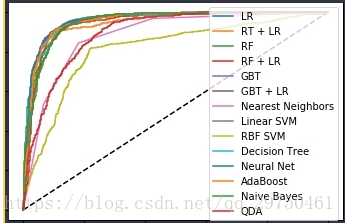
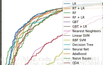
4.7 ROC值的计算与plot

plt.figure(1)plt.plot([0, 1], [0, 1], ’k--’)plt.plot(fpr_lm, tpr_lm, label=’LR’)plt.plot(fpr_rt_lm, tpr_rt_lm, label=’RT + LR’)plt.plot(fpr_rf, tpr_rf, label=’RF’)plt.plot(fpr_rf_lm, tpr_rf_lm, label=’RF + LR’)plt.plot(fpr_grd, tpr_grd, label=’GBT’)plt.plot(fpr_grd_lm, tpr_grd_lm, label=’GBT + LR’)# 8 款模型for (fpr,tpr),name in [[predictEight[n][’fpr_tpr’],n] for n in names] : plt.plot(fpr, tpr, label=name) plt.xlabel(’False positive rate’)plt.ylabel(’True positive rate’)plt.title(’ROC curve’)plt.legend(loc=’best’)plt.show() plt.figure(2)plt.xlim(0, 0.2)plt.ylim(0.4, 1) # ylim改变 # mattplt.plot([0, 1], [0, 1], ’k--’)plt.plot(fpr_lm, tpr_lm, label=’LR’)plt.plot(fpr_rt_lm, tpr_rt_lm, label=’RT + LR’)plt.plot(fpr_rf, tpr_rf, label=’RF’)plt.plot(fpr_rf_lm, tpr_rf_lm, label=’RF + LR’)plt.plot(fpr_grd, tpr_grd, label=’GBT’)plt.plot(fpr_grd_lm, tpr_grd_lm, label=’GBT + LR’)for (fpr,tpr),name in [[predictEight[n][’fpr_tpr’],n] for n in names] : plt.plot(fpr, tpr, label=name)plt.xlabel(’False positive rate’)plt.ylabel(’True positive rate’)plt.title(’ROC curve (zoomed in at top left)’)plt.legend(loc=’best’)plt.show()

到此这篇关于一文搞懂Python Sklearn库使用方法的文章就介绍到这了,更多相关Python Sklearn库内容请搜索ABC学习网以前的文章或继续浏览下面的相关文章希望大家以后多多支持ABC学习网！

(window.slotbydup = window.slotbydup || []).push({id: "u6915441",container: "_5rmj5io5v3i",async: true});